| Bibliography | Background | Hypotheses | Home | |
| Bibliography | Background | Hypotheses | Home | |
![]()
Since 1990, all agencies in northern California have used habitat typing methods originally described by Bisson et al. (1981) to gather data on many fish habitat parameters. More recent publications (McCain et al. 1990, Hawkins et al. 1994) have clarified the hierarchical system of habitat classification that allows one to look at stream habitat as a simple sequence of pools and riffles (level 1), a sequence of pools, riffles, and runs (level 2), or as assemblages of more than twenty types of habitat types (level 3) that stem from the basic types of units. This classification system allows one to stratify (i.e. respect natural patterns of variation) when attempting to quantify biological or physical attributes of the stream. For example, Hankin and Reeves (1984) found that the precision of stream fish population surveys could be drastically improved by using habitat typing information. The habitat typing results alone can be used as indicator of fish habitat condition.
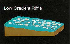
The California Department of Fish and Game Salmonid Habitat Restoration Manual (1998) provides habitat typing protocols which are largely derived from McCain et al. (1990). The McCain et al (1990) method breaks stream habitats into 22 types, including the four types illustrated below for the purpose of example. In addition to classifying habitat types and measuring habitat units, typical surveys also gauge gravel quality, cover, shade canopy, pool depth and bank condition. Fish counts by snorkeler or electrofishing are often done in conjunction with these surveys, but in the case of the California Department of Fish and Game, these biological inventories are typically done without the methods that enable quantification of fish density or population size.
|
|
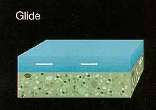
| Riffles are areas of swifter flowing water, where the surface is turbulent. Young-of-the-year steelhead like low gradient riffles but coho generally do not. The flowing water delivers insects for food and the broken surface provides cover from predators. | Glides are slow moving areas in the stream, where the surface is smooth. Often, streams suffering from cumulative watershed effects have a large percentage of flatwater habitats, such as glides and runs, and riffles. Pools often have filled in and represent a small percentage of habitat types. |
|
|
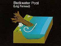
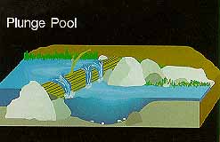
| Logs, root wads, boulders or stream banks can cause backwater pools to form as water swirls around the obstacle. Coho salmon almost always rear in pools formed by large wood. | Plunge pools are formed where water falls over a boulder or log. The falling water scours a hole where juvenile and adult fish often hide. |
![]()
Using Fish Habitat Data
Habitat typing surveys are a vast improvement from pre-1990 surveys by U.S. Forest Service and California Department of Fish and Game staff which often ranked fish habitat qualitatively as good, fair or poor and were of little utility for analysis. While habitat typing provides a useful inventory it is not a valid monitoring tool because categorization of habitat units may change with different crews doing the survey (Poole et al., 1997). Consequently, repeated habitat typing is not a valid way to monitor change in stream habitats over time. It is preferable to use habitat typing to help determine limiting factors and then choose quantitative monitoring tools. This does not mean, however, that habitat typing information cannot be used as a coarse indicator of potential limiting factors or general habitat conditions when doing watershed assessment.
Habitat typing provides tools for analysis of habitat diversity and suitability for salmon and steelhead. When substantial erosion occurs in a watershed, pool habitats diminish by aggradation (filling in) and spawning gravels become embedded (Madej, 1984). Good salmonid habitat is characterized by a diversity of pools, including lateral scour pools and those formed by large wood. Reeves et al. (1993) found that stream habitat in basins with low timber harvest levels (<25%) were more diverse than habitats in basins with high harvest levels (>25%). In paired comparisons, streams in low harvest basins had significantly more pieces of large wood per 100 m (2-12 times more) than streams in high harvest basins. Streams in low harvest basins also had 10-47% more pools per 100 m than did streams in high harvest basins.
A stream reach is rated as high quality habitat if it contains more than 30% pools by length in addition to other high ranking values including embeddedness less than 50% in most pool tail crests. Indices based on habitat length are more quantitative and useful than those based on habitat occurrence. Some important indices of fish habitat, such pool depths and percent canopy cover, are sensitive to stream size. In smaller streams of forested landscape, good habitat is associated with riparian canopy of at least 80% and a high component of conifers. Streams with intensive, recent watershed management often show a suite of conditions reflective of poor quality salmonid habitat: pools less than 30% pool frequency by length with dry stream reaches in highly aggraded streams, embeddedness of greater than 50% at all sites, few or no pools less than 3 feet in depth, and riparian canopies under 70%, often with a very small component of conifers.
As a reference, pool habitat surface area in undisturbed Washington coastal streams was 81% of the total stream surface area (Grette, 1985) and Alaska studies showed ranges of 39-67% pools (Murphy et al., 1984). The Washington State Fish and Wildlife Commission (1997) recommends the following pool frequencies by length: "For streams less than 15 meters wide, the percent pools should be greater than 55%, greater than 40% and greater than 30% for streams with gradients less than 2%, 2-5% and more than 5%, respectively." The North Coast Regional Water Quality Control Board (1999) recommends that pool frequency by length in the Noyo River exceed or equal 40%.
Brown et al. (1994) suggested that pools of one meter in depth or greater were necessary for successful rearing of coho salmon juveniles; therefore, KRIS Big River has broken down pool depth to discern how many pools deeper than three feet exist in surveyed areas. Older age steelhead also rely on pool habitat. Chen (1992) based cumulative effects models for the Elk River, Oregon on whether three-foot-deep pools were being maintained. His hypothesis was that if pools were greater than three feet they would support yearling steelhead.
![]()
Interpreting Habitat Data with Charts
CDFG habitat survey protocol involves classifying habitat units and describing 15 attributes for each unit, or a sample of each unit type. Some of these attributes are more relevant to understanding fish habitat conditions then others. Where survey data is available, KRIS charts show habitat frequency-by-length, maximum pool depth, pool tail embeddedness, and percent canopy cover. The chart style is designed to enable easy interpretation of conditions among streams at the watershed or basin scale. It is important to know, however, that differences among streams can be caused by differences in surveyors or physical features of the streams such as channel type, size, and gradient.
Habitat frequency can be used to roughly gauge problems of cumulative watershed effects on streams. Subsequent habitat surveys will find the stream dominated by riffles or shallow glides and runs. These flatwater habitats may still be suitable for young of the year steelhead, but young coho salmon require pools, preferably with large wood. Habitat typing summaries in KRIS combine the 22 total habitat types into four simpler categories: pools, riffles, flat water habitats and dry areas. These are consistent with CDFG level II habitat types. Habitat frequency by length is used instead of percent occurrence because the latter has less relevance to habitat availability and is less sensitive to cumulative effects. For example, streams that are aggraded (filled in) may still have numerous of pools of short length and a few very long runs and riffles.
|
This chart shows the percent by length of the four basic habitat types for each stream surveyed in the North Fork Big River. The "Dry" type of habitat describes dewatered riffles and is, by proportion and index of potential limits to fish habitat by low flows. The percent pools in this sub-basin ranged from 19% (East Branch) to 41% (North Fork Big). Percent pools by length is naturally higher in lower gradient channels, but is also affected by large wood and sediment. See background pages on these topics for information on the factors which may be keeping pool frequency low. |
Maximum pool depth is a discrete attribute with minimally subjective criteria for evaluation in the field. Deeper pools provide better quality habitat for coho salmon. Pools less than three feet deep may not provide suitable habitat for coho salmon, and California Department of Fish and Game biologists target maximum pool depth at greater than three feet for third order streams.
|
Maximum pool depths in North Fork sub-basin streams are mostly less than 3 feet. This metric is sensitive to stream order. The similarly sized Chamberlain, East Branch, and James Creek have 15-25% pools greater than 3 feet. In streams as large as the NF Big, maximum pool depths greater than 4 feet may be a better indicator habitat condition. The NF Big River has approximately 16% pools greater than 4 feet in depth. |
Pool tail embeddedness is a simple but subjective means of evaluating salmonid spawning habitat quality in the field. Pools tail crests are measured visually to determine to what degree potential spawning gravels might be embedded (partially buried). The California Department of Fish and Game (1998) categorize gravels less than 25% embedded as optimal for salmonid spawning. Other categories are 25-50%, 50-75% and greater than 75%. A fifth category is used to classify pool tails that are unsuitable for spawning. It is not clear if pool tails receiving this category may also be highly embedded, or if they should be omitted from the sampling distribution for analysis, as has been done for this chart.
|
This chart shows embeddedness ratings for the North Fork Big River and tributaries. High quality spawning habitat (blue bars) varied in occurrence from 8-23% of pool tails. The data indicates that embeddedness was higher in West Chamberlain Creek than other streams in that sub-basin. |
Canopy is an indicator of whether the cool microclimate necessary for moderating water temperatures is present and also whether there is a large wood supply for recruitment into the stream (Poole and Berman, 2000). Even if there is a high shade component, deciduous canopy cover may be less able to provide a cool microclimate over the stream than a multi-tiered coniferous over-story.
|
This chart shows the percentages of coniferous, deciduous, and open canopy from surveyed streams of the North Fork Big River. Most streams have less than 20% open canopy. The lower coniferous canopy and higher open canopy in James Creek and NF James Creek is expected based on their larger size. |
![]()
Analysis of Habitat Inventory Data
Stream inventories following CDFG protocols lead to databases of habitat metrics that can be very powerful for understanding habitat conditions. Byrne (1997) devised a mapping technique for spatially registering these data so that results of the survey can be viewed in ArcView or other GIS software. In optimistic support of the North Coast Watershed Assessment Program, KRIS Developers designed a utility for providing easy summary and charting of CDFG to accompany map outputs. Despite such available tools, CDFG stream inventories typically result in the production only of reports that discuss what kind of restoration activities are appropriate for the stream. The database underlying those reports is usually not made available due to concerns by CDFG regarding how use of such data may violate landowner's trust of the agency staff and subsequent denials of access to streams.
Where the full set of stream inventory data has been available for use in KRIS (e.g. Big River) charts and maps can be easily produced to provide all available information for interpreting and analyzing fish habitat conditions. To assuage concerns regarding the trust relationship between CDFG and landowners, memo fields can be stripped from the shared database. Memo fields are where inappropriate or casual comments may be stored. If it is deemed important and valid to not identify habitat conditions at a unit level, but instead only summarize conditions at a stream reach level, map products can be limited to this scale.
 |
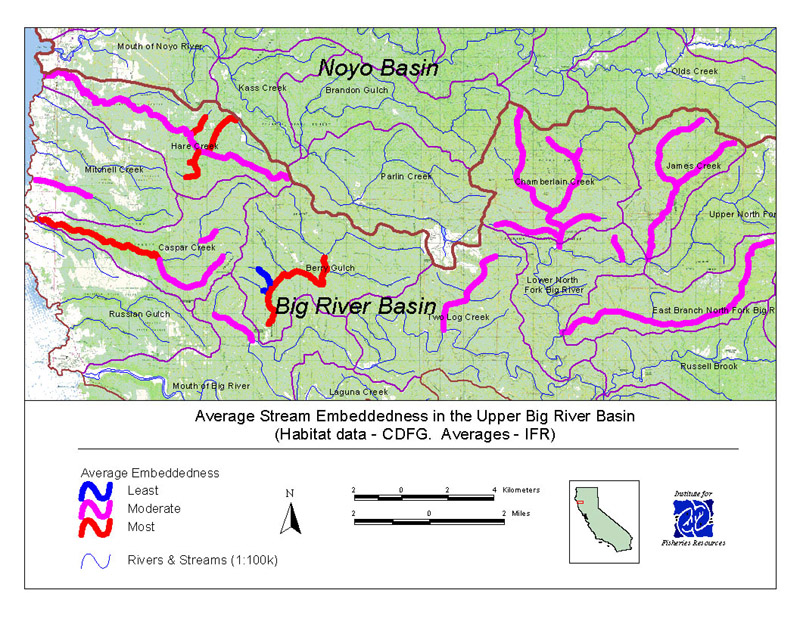 |
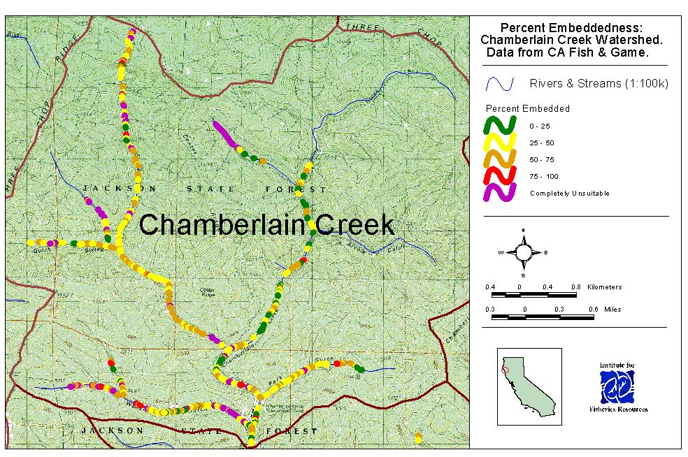
| This map shows each unit in the surveyed streams of the Chamberlain Creek watershed where embeddedness was surveyed by CDFG crews. The four different levels of embeddedness are shown by color. One can see, from this map, the spatial distribution of less embedded units (green) and more highly embedded units (red). | This map shows average embeddedness for each stream segment surveyed in the Big River area. The information is not very useful for understanding the actual distribution of spawning habitat or cumulative effects but is somewhat useful for examining differences among various streams. |
KRIS Big River provides multiple ways to examine habitat inventory data. The exercises have yielded some important results concerning the quality of data and appropriate types of summary. Average values are commonly used in analysis, but it is important to remember that averages are minimally descriptive of the dataset, and are influenced by errors or outliers. The box-plot or box-whisker plot is a chart style suited for examining the distribution of data points, and provides much more information than an average, median, or any other single parameter. Box-plots describe the distribution of data for a single attribute, and can be used to compare that attribute across many streams. Box-plots in KRIS use the following seven parameters: the 5th percentile (Q5), the 10th percentile (Q10), the 25th percentile (Q25), the 50th percentile or median (Q50), the 75th percentile (Q75), the 90th percentile (Q90), and the 95th percentile (Q95). Box-plots can be easily prepared from raw data in KRIS by using the Build Table utility to first build the appropriate chart table.
Box-plots enable one to visually assess what streams provide a certain percentage of habitat in a condition greater or less than a specified value. Such visual assessment of data can be useful when exploring the relative condition of habitat in streams with regard to various targets. Examples are presented below.
|
The box-plot chart at left shows the distribution of maximum depth values measured for each moderate to large stream surveyed in the Big River area. Streams are arrayed by size: NF Caspar through West Chamberlain are 3rd order, Caspar through Chamberlain are fourth order. Only Caspar and Hare Creeks had more than 25% of pools measuring greater than 3.0 feet in depth. Median values ranged from 1.2 feet (NF Caspar) to 2.8 feet (Caspar). CDFG collected data during stream surveys in 1995-97. |
|
This box-whisker plot shows the distribution of percent canopy measurements for all streams surveyed in the Big River area. Streams are arrayed by size: MF Caspar through Johnson are 2nd order, NF Caspar through West Chamberlain are 3rd order, Caspar through Chamberlain are 4th order, and the NF Big is 5th order. While the occurrence of open canopy does correlate with stream size, trend outliers such as Snuffins, Soda, the East Branch NF, and James Creek indicate unusually open canopy. Caspar and Hare Creeks are shown with relatively high canopy cover conditions.. |
Exploration of CDFG habitat data has revealed a small percentage of values for some attributes that are outliers, and in many cases, the result of mistakes during data entry. Percent canopy is one attribute that had approximately 3% of values in error due to incorrect decimal positioning. Maximum depth had a slightly lower error rate due to the same problem. Box-plots are only negligibly influenced by these errors, when they comprise less than 5% of the dataset. By contrast, averages can be strongly influenced by such errors.
Special charts for exploring the distribution of datasets are also presented for residual pool depth, and shelter rating. These later attributes have uncertain value in assessing habitat conditions or as indicators of cumulative effects.
![]()
References
Bisson, P.A., J.L. Nielsen, R.A. Palmason and L.E. Grove. 1981. A system of naming habitat in small streams, with examples of habitat utilization by salmonids during low streamflow. In N.B. Armantrout ed. Acquisition and Utilization of Aquatic Habitat Inventory Information. Proceedings of a symposium, Oct. 28-30, 1981, Portland, Oregon. Hagen Publishing Co., Billings, Montana. pp. 62-73.
Brown, L.R., P.B. Moyle, and R.M. Yoshiyama. 1994. Historical Decline and Current Status of Coho Salmon in California. North American Journal of Fisheries Management. 14(2):237-261.
Byrne, M. 1997. California Salmonid Habitat Inventory: a Dynamic Segmentation Application. Earth Science Research Institute (ESRI), 1997 Annual Proceedings of ESRI Conference. CDFG, Inland Fisheries, Sacramento, CA.
Ca. Department of Fish and Game. 1998. California Salmonid Stream Habitat Restoration Manual. Third Edition. Inland Fisheries Division. California Department of Fish and Game. Sacramento, CA. 495 pp.
Chen, G. 1992. Use of Basin Survey Data in Habitat Modeling and Cumulative Watershed Effects Analysis. Siskiyou NF. Published as part of USDA Forest Service Region 5 Fish Habitat Relationship Technical Bulletin Series, No. 8.
Grette, G.B. 1985. The role of large organic debris in juvenile salmonid rearing habitat in small streams. Master's Thesis, University of Washington, Seattle, WA.
Hankin, D. G., and G. H. Reeves. 1988. Estimating total fish abundance and total habitat area in small streams based on visual estimation methods. Canadian Journal of Fisheries and Aquatic Sciences 45: 834-844.
Hawkins, C.P., and 10 coauthors. 1993. A hierarchical approach to classifying stream habitat features. Fisheries 18(6): 3-12.Madej, M.A. 1984. Recent changes in channel-stored sediment Redwood Creek, California. Redwood National Park Research and Development Technical Report 11. National Park Service, Arcata, CA. 54 p.
Mangelsdorf, A. and L. Clyde. 2000. Draft (through Chapter 4-Ten Mile River). Assessment of aquatic conditions in the Mendocino Coast Hydrologic Unit. California Regional Water Resources Control Board. North Coast Region. Santa Rosa, CA. 120 pp.
McCain, M., D.Fuller, L.Decker and K.Overton. 1990 . Stream habitat classification and inventory procedures for northern California. FHC Currents. No.1. U.S. Department of Agriculture. Forest Service, Pacific Southwest Region.
Murphy, M.L., J.F. Thedinga, K.V. Koski and G.B. Grette. 1984. A stream ecosystem in an old growth forest in southeast Alaska: Part V. Seasonal changes in habitat utilization by juvenile salmonids. In Proceedings of Symposium on Fish and Wildlife in Relationships in Old Growth Forests. Eds. W.R. Meehan, T.R. Merrill and T.A. Hanley. American Institute of Fishery Research Biologists, Asheville, North Carolina.
North Coast Regional Water Quality Control Board. 1999. Noyo River Watershed Total Maximum Daily Load for Sediment. NCRWQCB, Santa Rosa, CA.
Poole, G.C., C.A. Frissell and S.C. Ralph. 1997. In-stream habitat unit classification: Inadequacies for monitoring and some consequences for management. Journal of the American Water Resources Association. Vol 33, No.4. August 1997.
Reeves, G.H., F.H. Everest and J.R. Sedell. 1993 . Diversity of Juvenile Anadromous Salmonid Assemblages in Coastal Oregon Basins with Different Levels of Timber Harvest. Transactions of the American Fisheries Society. Vol 122, No. 3. May 1993.
Washington Fish and Game Commission. 1997. Policy of the Washington Department of Fish and Wildlife and Western Washington Treaty Tribes on Wild Salmonids. Washington Fish and Game Commission, Olympia, WA. 68 p.
![]()
|
Table of Contents for Background Pages |
|||||
| Stream Conditions: | Water Quality | Sediment | Riparian | Big Wood | Habitat Types |
| Watershed Conditions: | Vegetation Types | Slope Stability | Roads & Erosion | Cumulative Impacts | Urbanization |
| Fish & Aquatic Life: | Fish Populations | Amphibians | Aquatic Insects | Hatcheries | Fish Disease |
| Restoration: | Stream Clearance | In-stream Structures | Riparian | Watershed | Strategy |
| Geology / Hydrology: | Geology | Soils | Precipitation | Stream Flow | Channel Processes |
| Policy & Regulation | ESA | TMDL | Forest Rules | 1603 Permits | Water Rights |
| www.krisweb.com |